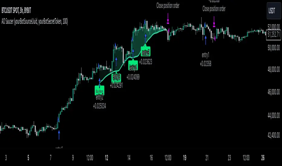
MultiLayer Awesome Oscillator Saucer Strategy [Skyrexio]Overview
MultiLayer Awesome Oscillator Saucer Strategy leverages the combination of Awesome Oscillator (AO), Williams Alligator, Williams Fractals and Exponential Moving Average (EMA) to obtain the high probability long setups. Moreover, strategy uses multi trades system, adding funds to long position if it considered that current trend has likely became stronger. Awesome Oscillator is used for creating signals, while Alligator and Fractal are used in conjunction as an approximation of short-term trend to filter them. At the same time EMA (default EMA's period = 100) is used as high probability long-term trend filter to open long trades only if it considers current price action as an uptrend. More information in "Methodology" and "Justification of Methodology" paragraphs. The strategy opens only long trades.
Unique Features
No fixed stop-loss and take profit: Instead of fixed stop-loss level strategy utilizes technical condition obtained by Fractals and Alligator to identify when current uptrend is likely to be over (more information in "Methodology" and "Justification of Methodology" paragraphs)
Configurable Trading Periods: Users can tailor the strategy to specific market windows, adapting to different market conditions.
Multilayer trades opening system: strategy uses only 10% of capital in every trade and open up to 5 trades at the same time if script consider current trend as strong one.
Short and long term trend trade filters: strategy uses EMA as high probability long-term trend filter and Alligator and Fractal combination as a short-term one.
Methodology
The strategy opens long trade when the following price met the conditions:
1. Price closed above EMA (by default, period = 100). Crossover is not obligatory.
2. Combination of Alligator and Williams Fractals shall consider current trend as an upward (all details in "Justification of Methodology" paragraph)
3. Awesome Oscillator shall create the "Saucer" long signal (all details in "Justification of Methodology" paragraph). Buy stop order is placed one tick above the candle's high of last created "Saucer signal".
4. If price reaches the order price, long position is opened with 10% of capital.
5. If currently we have opened position and price creates and hit the order price of another one "Saucer" signal another one long position will be added to the previous with another one 10% of capital. Strategy allows to open up to 5 long trades simultaneously.
6. If combination of Alligator and Williams Fractals shall consider current trend has been changed from up to downtrend, all long trades will be closed, no matter how many trades has been opened.
Script also has additional visuals. If second long trade has been opened simultaneously the Alligator's teeth line is plotted with the green color. Also for every trade in a row from 2 to 5 the label "Buy More" is also plotted just below the teeth line. With every next simultaneously opened trade the green color of the space between teeth and price became less transparent.
Strategy settings
In the inputs window user can setup strategy setting: EMA Length (by default = 100, period of EMA, used for long-term trend filtering EMA calculation). User can choose the optimal parameters during backtesting on certain price chart.
Justification of Methodology
Let's go through all concepts used in this strategy to understand how they works together. Let's start from the easies one, the EMA. Let's briefly explain what is EMA. The Exponential Moving Average (EMA) is a type of moving average that gives more weight to recent prices, making it more responsive to current price changes compared to the Simple Moving Average (SMA). It is commonly used in technical analysis to identify trends and generate buy or sell signals. It can be calculated with the following steps:
1.Calculate the Smoothing Multiplier:
Multiplier = 2 / (n + 1), Where n is the number of periods.
2. EMA Calculation
EMA = (Current Price) × Multiplier + (Previous EMA) × (1 − Multiplier)
In this strategy uses EMA an initial long term trend filter. It allows to open long trades only if price close above EMA (by default 50 period). It increases the probability of taking long trades only in the direction of the trend.
Let's go to the next, short-term trend filter which consists of Alligator and Fractals. Let's briefly explain what do these indicators means. The Williams Alligator, developed by Bill Williams, is a technical indicator designed to spot trends and potential market reversals. It uses three smoothed moving averages, referred to as the jaw, teeth, and lips:
Jaw (Blue Line): The slowest of the three, based on a 13-period smoothed moving average shifted 8 bars ahead.
Teeth (Red Line): The medium-speed line, derived from an 8-period smoothed moving average shifted 5 bars forward.
Lips (Green Line): The fastest line, calculated using a 5-period smoothed moving average shifted 3 bars forward.
When these lines diverge and are properly aligned, the "alligator" is considered "awake," signaling a strong trend. Conversely, when the lines overlap or intertwine, the "alligator" is "asleep," indicating a range-bound or sideways market. This indicator assists traders in identifying when to act on or avoid trades.
The Williams Fractals, another tool introduced by Bill Williams, are used to pinpoint potential reversal points on a price chart. A fractal forms when there are at least five consecutive bars, with the middle bar displaying the highest high (for an up fractal) or the lowest low (for a down fractal), relative to the two bars on either side.
Key Points:
Up Fractal: Occurs when the middle bar has a higher high than the two preceding and two following bars, suggesting a potential downward reversal.
Down Fractal: Happens when the middle bar shows a lower low than the surrounding two bars, hinting at a possible upward reversal.
Traders often combine fractals with other indicators to confirm trends or reversals, improving the accuracy of trading decisions.
How we use their combination in this strategy? Let’s consider an uptrend example. A breakout above an up fractal can be interpreted as a bullish signal, indicating a high likelihood that an uptrend is beginning. Here's the reasoning: an up fractal represents a potential shift in market behavior. When the fractal forms, it reflects a pullback caused by traders selling, creating a temporary high. However, if the price manages to return to that fractal’s high and break through it, it suggests the market has "changed its mind" and a bullish trend is likely emerging.
The moment of the breakout marks the potential transition to an uptrend. It’s crucial to note that this breakout must occur above the Alligator's teeth line. If it happens below, the breakout isn’t valid, and the downtrend may still persist. The same logic applies inversely for down fractals in a downtrend scenario.
So, if last up fractal breakout was higher, than Alligator's teeth and it happened after last down fractal breakdown below teeth, algorithm considered current trend as an uptrend. During this uptrend long trades can be opened if signal was flashed. If during the uptrend price breaks down the down fractal below teeth line, strategy considered that uptrend is finished with the high probability and strategy closes all current long trades. This combination is used as a short term trend filter increasing the probability of opening profitable long trades in addition to EMA filter, described above.
Now let's talk about Awesome Oscillator's "Sauser" signals. Briefly explain what is the Awesome Oscillator. The Awesome Oscillator (AO), created by Bill Williams, is a momentum-based indicator that evaluates market momentum by comparing recent price activity to a broader historical context. It assists traders in identifying potential trend reversals and gauging trend strength.
AO = SMA5(Median Price) − SMA34(Median Price)
where:
Median Price = (High + Low) / 2
SMA5 = 5-period Simple Moving Average of the Median Price
SMA 34 = 34-period Simple Moving Average of the Median Price
Now we know what is AO, but what is the "Saucer" signal? This concept was introduced by Bill Williams, let's briefly explain it and how it's used by this strategy. Initially, this type of signal is a combination of the following AO bars: we need 3 bars in a row, the first one shall be higher than the second, the third bar also shall be higher, than second. All three bars shall be above the zero line of AO. The price bar, which corresponds to third "saucer's" bar is our signal bar. Strategy places buy stop order one tick above the price bar which corresponds to signal bar.
After that we can have the following scenarios.
Price hit the order on the next candle in this case strategy opened long with this price.
Price doesn't hit the order price, the next candle set lower low. If current AO bar is increasing buy stop order changes by the script to the high of this new bar plus one tick. This procedure repeats until price finally hit buy order or current AO bar become decreasing. In the second case buy order cancelled and strategy wait for the next "Saucer" signal.
If long trades has been opened strategy use all the next signals until number of trades doesn't exceed 5. All trades are closed when the trend changes to downtrend according to combination of Alligator and Fractals described above.
Why we use "Saucer" signals? If AO above the zero line there is a high probability that price now is in uptrend if we take into account our two trend filters. When we see the decreasing bars on AO and it's above zero it's likely can be considered as a pullback on the uptrend. When we see the stop of AO decreasing and the first increasing bar has been printed there is a high probability that this local pull back is finished and strategy open long trade in the likely direction of a main trend.
Why strategy use only 10% per signal? Sometimes we can see the false signals which appears on sideways. Not risking that much script use only 10% per signal. If the first long trade has been open and price continue going up and our trend approximation by Alligator and Fractals is uptrend, strategy add another one 10% of capital to every next saucer signal while number of active trades no more than 5. This capital allocation allows to take part in long trades when current uptrend is likely to be strong and use only 10% of capital when there is a high probability of sideways.
Backtest Results
Operating window: Date range of backtests is 2023.01.01 - 2024.11.25. It is chosen to let the strategy to close all opened positions.
Commission and Slippage: Includes a standard Binance commission of 0.1% and accounts for possible slippage over 5 ticks.
Initial capital: 10000 USDT
Percent of capital used in every trade: 10%
Maximum Single Position Loss: -5.10%
Maximum Single Profit: +22.80%
Net Profit: +2838.58 USDT (+28.39%)
Total Trades: 107 (42.99% win rate)
Profit Factor: 3.364
Maximum Accumulated Loss: 373.43 USDT (-2.98%)
Average Profit per Trade: 26.53 USDT (+2.40%)
Average Trade Duration: 78 hours
These results are obtained with realistic parameters representing trading conditions observed at major exchanges such as Binance and with realistic trading portfolio usage parameters.
How to Use
Add the script to favorites for easy access.
Apply to the desired timeframe and chart (optimal performance observed on 3h BTC/USDT).
Configure settings using the dropdown choice list in the built-in menu.
Set up alerts to automate strategy positions through web hook with the text: {{strategy.order.alert_message}}
Disclaimer:
Educational and informational tool reflecting Skyrex commitment to informed trading. Past performance does not guarantee future results. Test strategies in a simulated environment before live implementation
ابحث في النصوص البرمجية عن "take profit"
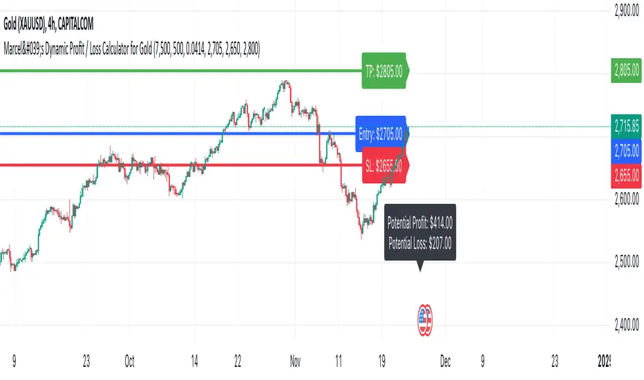
Marcel's Dynamic Profit / Loss Calculator for GoldOverview
This Dynamic Risk / Reward Tool for Gold is designed to help traders efficiently plan and manage their trades in the volatile gold market. This script provides a clear visualisation of trade levels (Entry, Stop Loss, Take Profit) while dynamically calculating potential profit and loss. It ensures gold traders can assess their positions with precision, saving time and improving risk management.
Key Features
1. Trade Level Visualisation:
Plots Entry (Blue), Stop Loss (Red), and Take Profit (Green) lines directly on the chart.
Helps you visualise and confirm trade setups quickly which is good for scalping and day trades.
2. Dynamic Risk and Reward Calculations:
Calculates potential profit and loss in real time based on user-defined inputs such as position size, leverage, and account equity.
Displays a summary panel showing risk/reward metrics directly on the chart.
3. Customisable Settings:
Allows you to adjust key parameters like account equity, position size, leverage, and specific price levels for Entry, Stop Loss, and Take Profit.
Defaults are dynamically generated for convenience but remain fully adjustable for flexibility.
How It Works
The script uses gold-specific conventions (e.g., 1 lot = 100 ounces, 1 pip = 0.01 price change) to calculate accurate risk and reward metrics.
It dynamically positions Stop Loss and Take Profit levels relative to the entry price, based on user-defined or default offsets.
A real-time summary panel is displayed in the bottom-right corner of the chart, showing:
Potential Profit: The monetary value if the Take Profit is hit.
Potential Lo
ss: The monetary value if the Stop Loss is hit.
How to Use It
1. Add the script to your chart on a gold trading pair (e.g., XAUUSD).
2. Input your:
Account equity.
Leverage.
Position size (in lots).
Desired En
try Price (default: current close price).
3. Adjust the Stop Loss and Take Profit levels to your strategy, or let the script use default offsets of:
500 pips below the Entry for Stop Loss.
1000 pips above the Entry for Take Profit.
4. Review the plotted levels and the summary panel to confirm your trade aligns with your risk/reward goals.
Why Use This Tool?
Clarity and Precision:
Provides clear trade visuals and financial metrics for confident decision-making.
Time-Saving:
Automates the calculations needed to evaluate trade risk and reward.
Improved Risk Management:
Ensures you never trade without knowing your exact potential loss and gain.
This script is particularly useful for both novice and experienced traders looking to enhance their risk management and trading discipline in the Gold market. Enjoy clearer trades at speed.
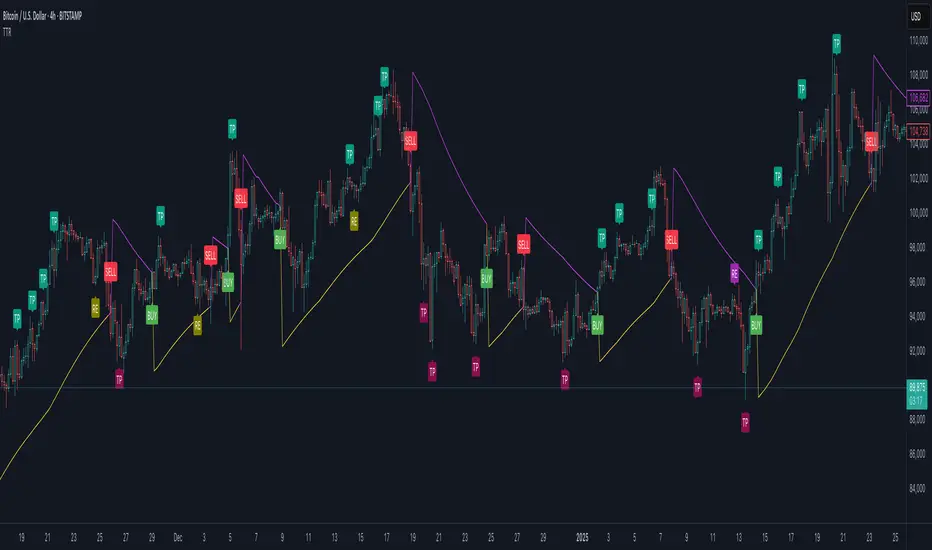
Trend Trader-RemasteredThe script was originally coded in 2018 with Pine Script version 3, and it was in invite only status. It has been updated and optimised for Pine Script v5 and made completely open source.
Overview
The Trend Trader-Remastered is a refined and highly sophisticated implementation of the Parabolic SAR designed to create strategic buy and sell entry signals, alongside precision take profit and re-entry signals based on marked Bill Williams (BW) fractals. Built with a deep emphasis on clarity and accuracy, this indicator ensures that only relevant and meaningful signals are generated, eliminating any unnecessary entries or exits.
Key Features
1) Parabolic SAR-Based Entry Signals:
This indicator leverages an advanced implementation of the Parabolic SAR to create clear buy and sell position entry signals.
The Parabolic SAR detects potential trend shifts, helping traders make timely entries in trending markets.
These entries are strategically aligned to maximise trend-following opportunities and minimise whipsaw trades, providing an effective approach for trend traders.
2) Take Profit and Re-Entry Signals with BW Fractals:
The indicator goes beyond simple entry and exit signals by integrating BW Fractal-based take profit and re-entry signals.
Relevant Signal Generation: The indicator maintains strict criteria for signal relevance, ensuring that a re-entry signal is only generated if there has been a preceding take profit signal in the respective position. This prevents any misleading or premature re-entry signals.
Progressive Take Profit Signals: The script generates multiple take profit signals sequentially in alignment with prior take profit levels. For instance, in a buy position initiated at a price of 100, the first take profit might occur at 110. Any subsequent take profit signals will then occur at prices greater than 110, ensuring they are "in favour" of the original position's trajectory and previous take profits.
3) Consistent Trend-Following Structure:
This design allows the Trend Trader-Remastered to continue signaling take profit opportunities as the trend advances. The indicator only generates take profit signals in alignment with previous ones, supporting a systematic and profit-maximising strategy.
This structure helps traders maintain positions effectively, securing incremental profits as the trend progresses.
4) Customisability and Usability:
Adjustable Parameters: Users can configure key settings, including sensitivity to the Parabolic SAR and fractal identification. This allows flexibility to fine-tune the indicator according to different market conditions or trading styles.
User-Friendly Alerts: The indicator provides clear visual signals on the chart, along with optional alerts to notify traders of new buy, sell, take profit, or re-entry opportunities in real-time.
ATT Model with Buy/Sell SignalsIndicator Summary
This indicator is based on the ATT (Arithmetic Time Theory) model, using specific turning points derived from the ATT sequence (3, 11, 17, 29, 41, 47, 53, 59) to identify potential market reversals. It also integrates the RSI (Relative Strength Index) to confirm overbought and oversold conditions, triggering buy and sell signals when conditions align with the ATT sequence and RSI level.
Turning Points: Detected based on the ATT sequence applied to bar count. This suggests high-probability areas where the market could turn.
RSI Filter: Adds strength to the signals by ensuring buy signals occur when RSI is oversold (<30) and sell signals when RSI is overbought (>70).
Max Signals Per Session: Limits signals to two per session to reduce over-trading.
Entry Criteria
Buy Signal: Enter a buy trade if:
The indicator displays a green "BUY" marker.
RSI is below the oversold level (default <30), suggesting a potential upward reversal.
Sell Signal: Enter a sell trade if:
The indicator displays a red "SELL" marker.
RSI is above the overbought level (default >70), indicating a potential downward reversal.
Exit Criteria
Take Profit (TP):
Define TP as a fixed percentage or point value based on the asset's volatility. For example, set TP at 1.5-2x the risk, or a predefined point target (like 50-100 points).
Alternatively, exit the position when price approaches a key support/resistance level or the next significant swing high/low.
Stop Loss (SL):
Place the SL below the recent low (for buys) or above the recent high (for sells).
Set a fixed SL in points or percentage based on the asset’s average movement range, like an ATR-based stop, or limit it to a specific risk amount per trade (1-2% of account).
Trailing into Profit
Use a trailing strategy to lock in profits and let winning trades run further. Two main options:
ATR Trailing Stop:
Set the trailing stop based on the ATR (Average True Range), adjusting every time a new candle closes. This can help in volatile markets by keeping the stop at a consistent distance based on recent price movement.
Break-Even and Partial Profits:
When the price moves in your favor by a set amount (e.g., 1:1 risk/reward), move SL to the entry (break-even).
Take partial profit at intermediate levels (e.g., 50% at 1:1 RR) and trail the remainder.
Risk Management for Prop Firm Evaluation
Prop firms often have strict rules on daily loss limits, max drawdowns, and minimum profit targets. Here’s how to align your strategy with these:
Limit Risk per Trade:
Keep risk per trade to a conservative level (e.g., 1% or lower of your account balance). This allows for more room in case of a drawdown and aligns with most prop firm requirements.
Daily Loss Limits:
Set a daily stop-loss that ensures you don’t exceed the firm’s rules. For example, if the daily limit is 5%, stop trading once you reach a 3-4% drawdown.
Avoid Over-Trading:
Stick to the max signals per session rule (one or two trades). Taking only high-probability setups reduces emotional and reactive trades, preserving capital.
Stick to a Profit Target:
Aim to meet the evaluation’s profit goal efficiently but avoid risky or oversized trades to reach it faster.
Avoid Major Economic Events:
News events can disrupt technical setups. Avoid trading around significant releases (like FOMC or NFP) to reduce the chance of sudden losses due to high volatility.
Summary
Using this strategy with discipline, a structured entry/exit approach, and tight risk management can maximize your chances of passing a prop firm evaluation. The ATT model’s turning points, combined with the RSI, provide an edge by highlighting reversal zones, while limiting trades to 1-2 per session helps maintain controlled risk.

Dynamic Trading Strategy with Key Levels, Entry/Exit ManagementThis indicator provides a complete rule-based trading system, combining key levels, entry conditions, stop loss (SL), and take profit (TP) management. It’s designed to dynamically adapt to market conditions by identifying crucial support and resistance zones, determining entry points based on price action and volume, and calculating risk-based exit targets.
Key Features
Key Level Identification:
The indicator automatically identifies support and resistance levels based on recent price highs and lows within a customizable lookback period.
It adds a dynamic buffer around these levels using the Average True Range (ATR) to account for market volatility, ensuring the zones adjust to changing conditions.
Entry Conditions:
Bullish Entry: Triggers near the support zone when there’s upward price action, confirmed by volume spikes and bullish candlestick patterns (e.g., hammers, engulfing candles).
Bearish Entry: Triggers near the resistance zone when signs of rejection appear, confirmed by volume spikes and bearish candlestick patterns (e.g., shooting stars, bearish engulfing).
Entry zones are highlighted visually on the chart using green (bullish) and red (bearish) shaded boxes.
Stop Loss (SL) and Take Profit (TP):
Stop Loss: Calculated based on ATR multipliers, allowing you to set a volatility-adjusted risk level beyond the entry range.
Take Profit: Includes two profit-taking levels (TP1 and TP2), allowing for partial position exits. TP levels are calculated based on a reward-to-risk ratio, ensuring consistent profitability targets.
SL and TP levels are clearly marked with horizontal lines and labeled as SL, TP1, and TP2, helping you manage trade exits effectively.
Market Context Adaptability:
The indicator adapts to both trending and ranging market conditions. In trending markets, it favors trades that follow the trend, while in ranging markets, it focuses on reversals within the range boundaries.
Visual Aids:
Entry zones are highlighted with shaded boxes to indicate potential buy/sell regions.
SL, TP1, and TP2 levels are clearly drawn with labels, allowing for easy identification of exit points.
How to Use
Identify Key Levels: Look for support and resistance zones highlighted by the indicator on your chart.
Wait for Entry Conditions: When the price enters the entry range (marked by green or red boxes), wait for confirmation signals—such as volume spikes and candlestick patterns.
Manage Exits: Use the SL, TP1, and TP2 levels for structured trade management. Consider scaling out partially at TP1 and exiting fully at TP2.
Ideal For:
This indicator is suitable for traders who prefer a systematic approach to trading, with clear entry and exit rules. It is particularly helpful for those looking to balance risk and reward with well-defined take profit and stop loss levels.

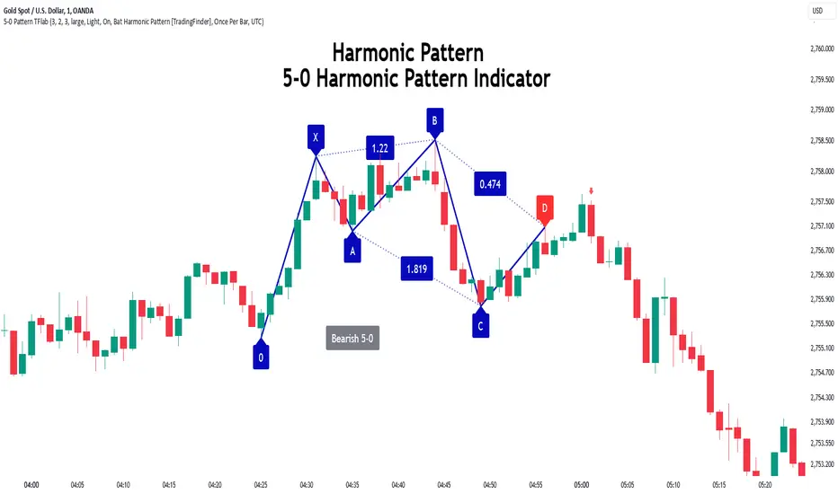
5-0 Harmonic Pattern [TradingFinder] 0XABCD 50 Harmonic Detector🔵 Introduction
Harmonic patterns are a powerful tool in technical analysis, widely used to detect reversal points and trend changes. Among these, the 5-0 Harmonic Pattern stands out due to its reliance on specific Fibonacci ratios—1.13, 1.618, 2.24, and 0.45 to 0.55—anchored at points 0, X, A, B, C, and D. This pattern provides a structured approach for identifying critical buy and sell points, helping traders achieve optimal entry and exit levels in volatile markets.
This 5-0 Harmonic Pattern indicator automatically detects and marks bullish and bearish formations on the chart, offering precise trading signals based on established harmonic ratios. With its dynamic signals, the 5-0 pattern enables traders to anticipate market movements and capitalize on favorable price trends.
Especially in fast-moving markets, harmonic patterns, particularly the 5-0 Harmonic Pattern, equip traders with an essential framework for identifying reversal opportunities and refining their trading strategies.
Bullish 5-0 Pattern :
Bearish 5-0 Pattern :
🔵 How to Use
The 5-0 Harmonic Pattern indicator is designed to automatically mark the key levels of the harmonic structure: 0, X, A, B, C, and D. By doing so, it detects both bullish and bearish patterns and helps traders recognize optimal entry and exit points.
Formed through specific Fibonacci levels, this pattern signals potential shifts in trend direction, giving traders critical insights for managing entries and exits effectively. The tool proves valuable in high-volatility settings, enabling traders to leverage these signals for refined decision-making.
🟣 Bullish 5-0 Pattern
A bullish 5-0 pattern materializes when Fibonacci levels indicate a potential price reversal to the upside. With points 0, X, A, B, C, and D in alignment, the indicator highlights this upward momentum by displaying a green arrow as a buy signal on the chart. This marking provides a clear entry point, indicating that prices are likely to rise, making it a prime moment for traders to enter long positions.
Additionally, the bullish 5-0 pattern is equipped with tools for traders to set stop-loss and take-profit points based on harmonic lines within the pattern, which represent support and resistance levels. Using these dynamic points, traders can create a more effective risk-reward setup while following the bullish signals in a standalone harmonic strategy.
🟣 Bearish 5-0 Pattern
The bearish 5-0 pattern functions similarly but signals a likely downturn. This pattern emerges when Fibonacci ratios align at points 0, X, A, B, C, and D, predicting a reversal downward. The indicator generates a sell signal, marked by a red arrow, prompting traders to exit long positions or initiate short trades to capitalize on falling prices.
Traders can utilize this bearish pattern for defining exit strategies and setting key levels for stop-loss and take-profit orders. The bearish 5-0 pattern enhances traders’ abilities to gauge critical price levels and manage trade risk effectively, especially in volatile markets. For traders focused on profiting from downward trends, this indicator serves as a powerful tool for timely entries and exits.
🔵 Setting
🟣 Logical Setting
ZigZag Pivot Period : You can adjust the period so that the harmonic patterns are adjusted according to the pivot period you want. This factor is the most important parameter in pattern recognition.
Show Valid Forma t: If this parameter is on "On" mode, only patterns will be displayed that they have exact format and no noise can be seen in them. If "Off" is, the patterns displayed that maybe are noisy and do not exactly correspond to the original pattern.
Show Formation Last Pivot Confirm : if Turned on, you can see this ability of patterns when their last pivot is formed. If this feature is off, it will see the patterns as soon as they are formed. The advantage of this option being clear is less formation of fielded patterns, and it is accompanied by the latest pattern seeing and a sharp reduction in reward to risk.
Period of Formation Last Pivot : Using this parameter you can determine that the last pivot is based on Pivot period.
🟣 Genaral Setting
Show : Enter "On" to display the template and "Off" to not display the template.
Color : Enter the desired color to draw the pattern in this parameter.
LineWidth : You can enter the number 1 or numbers higher than one to adjust the thickness of the drawing lines. This number must be an integer and increases with increasing thickness.
LabelSize : You can adjust the size of the labels by using the "size.auto", "size.tiny", "size.smal", "size.normal", "size.large" or "size.huge" entries.
🟣 Alert Setting
Alert : On / Off
Message Frequency : This string parameter defines the announcement frequency. Choices include: "All" (activates the alert every time the function is called), "Once Per Bar" (activates the alert only on the first call within the bar), and "Once Per Bar Close" (the alert is activated only by a call at the last script execution of the real-time bar upon closing). The default setting is "Once per Bar".
Show Alert Time by Time Zone : The date, hour, and minute you receive in alert messages can be based on any time zone you choose. For example, if you want New York time, you should enter "UTC-4". This input is set to the time zone "UTC" by default.
Conclusion
The 5-0 Harmonic Pattern indicator serves as a robust solution for technical analysts and traders looking to pinpoint market reversal points. By automatically recognizing 5-0 patterns and generating buy and sell signals based on Fibonacci ratios, this tool supports precise trend analysis and entry/exit timing. The indicator’s adjustable alerts, color themes, and pattern toggles allow for comprehensive customization, ensuring alignment with individual trading strategies.
Harmonic patterns, especially the 5-0 Harmonic Pattern, guide traders in identifying high-accuracy entry and exit points, thus aiding in more informed trading decisions. By combining Fibonacci ratio analysis with real-time signal updates, this indicator provides a well-rounded approach for risk management and capitalizing on trading opportunities. Professional traders can harness this tool to enhance technical analysis precision and capitalize on price trends effectively, maximizing profitability in both bullish and bearish markets.
Simple RSI stock Strategy [1D] The "Simple RSI Stock Strategy " is designed to long-term traders. Strategy uses a daily time frame to capitalize on signals generated by the Relative Strength Index (RSI) and the Simple Moving Average (SMA). This strategy is suitable for low-leverage trading environments and focuses on identifying potential buy opportunities when the market is oversold, while incorporating strong risk management with both dynamic and static Stop Loss mechanisms.
This strategy is recommended for use with a relatively small amount of capital and is best applied by diversifying across multiple stocks in a strong uptrend, particularly in the S&P 500 stock market. It is specifically designed for equities, and may not perform well in other markets such as commodities, forex, or cryptocurrencies, where different market dynamics and volatility patterns apply.
Indicators Used in the Strategy:
1. RSI (Relative Strength Index):
- The RSI is a momentum oscillator used to identify overbought and oversold conditions in the market.
- This strategy enters long positions when the RSI drops below the oversold level (default: 30), indicating a potential buying opportunity.
- It focuses on oversold conditions but uses a filter (SMA 200) to ensure trades are only made in the context of an overall uptrend.
2. SMA 200 (Simple Moving Average):
- The 200-period SMA serves as a trend filter, ensuring that trades are only executed when the price is above the SMA, signaling a bullish market.
- This filter helps to avoid entering trades in a downtrend, thereby reducing the risk of holding positions in a declining market.
3. ATR (Average True Range):
- The ATR is used to measure market volatility and is instrumental in setting the Stop Loss.
- By multiplying the ATR value by a custom multiplier (default: 1.5), the strategy dynamically adjusts the Stop Loss level based on market volatility, allowing for flexibility in risk management.
How the Strategy Works:
Entry Signals:
The strategy opens long positions when RSI indicates that the market is oversold (below 30), and the price is above the 200-period SMA. This ensures that the strategy buys into potential market bottoms within the context of a long-term uptrend.
Take Profit Levels:
The strategy defines three distinct Take Profit (TP) levels:
TP 1: A 5% from the entry price.
TP 2: A 10% from the entry price.
TP 3: A 15% from the entry price.
As each TP level is reached, the strategy closes portions of the position to secure profits: 33% of the position is closed at TP 1, 66% at TP 2, and 100% at TP 3.
Visualizing Target Points:
The strategy provides visual feedback by plotting plotshapes at each Take Profit level (TP 1, TP 2, TP 3). This allows traders to easily see the target profit levels on the chart, making it easier to monitor and manage positions as they approach key profit-taking areas.
Stop Loss Mechanism:
The strategy uses a dual Stop Loss system to effectively manage risk:
ATR Trailing Stop: This dynamic Stop Loss adjusts based on the ATR value and trails the price as the position moves in the trader’s favor. If a price reversal occurs and the market begins to trend downward, the trailing stop closes the position, locking in gains or minimizing losses.
Basic Stop Loss: Additionally, a fixed Stop Loss is set at 25%, limiting potential losses. This basic Stop Loss serves as a safeguard, automatically closing the position if the price drops 25% from the entry point. This higher Stop Loss is designed specifically for low-leverage trading, allowing more room for market fluctuations without prematurely closing positions.
to determine the level of stop loss and target point I used a piece of code by RafaelZioni, here is the script from which a piece of code was taken
Together, these mechanisms ensure that the strategy dynamically manages risk while offering robust protection against significant losses in case of sharp market downturns.
The position size has been estimated by me at 75% of the total capital. For optimal capital allocation, a recommended value based on the Kelly Criterion, which is calculated to be 59.13% of the total capital per trade, can also be considered.
Enjoy !

Advanced Position Management [Mr_Rakun]Advanced Position Management
This Pine Script code is for a strategy titled "Advanced Position Management," aimed at effective trade execution and management using multiple take profit levels, trailing stop loss, and dynamic position sizing.
Take Profit Levels: It defines up to three take profit (TP) levels, allowing partial position exits at different price thresholds. The take profit levels and their respective quantities are adjustable using inputs.
Stop Loss and Trailing Stop: The script implements an initial stop loss based on a percentage from the entry price. Additionally, it features a trailing stop that moves based on either a percentage or previous TP levels, dynamically adjusting to maximize gains while protecting profits.
Position Size: The position size is customizable and based on USD value, allowing the trader to manage risk more effectively.
Advantages:
Flexibility: Multiple take profit levels and a dynamic stop loss system allow traders to lock in profits while keeping the position open for further gains.
Risk Management: The initial stop loss and trailing stop help to limit losses and protect profits as the trade moves in the desired direction.
Automation: Once the strategy is deployed, it automatically handles entry, exit, and stop management, reducing the need for constant monitoring.
------ TR ------
Gelişmiş Pozisyon Yönetimi
Bu Pine Script kodu, Gelişmiş Pozisyon Yönetimi için kendi stratejilerinize kolayca entegre edeceğiniz bir risk yönetimidir. Çoklu kâr al seviyeleri, takip eden stop-loss ve dinamik pozisyon büyüklüğü kullanarak işlem yürütme ve yönetiminde etkilidir.
Gelişmiş Pozisyon Yönetimi
Kâr Alma Seviyeleri;
Kod, pozisyonların farklı fiyat seviyelerinde kısmi kapatılmasını sağlayan üç farklı kâr alma (TP) seviyesini tanımlar. Bu kâr alma seviyeleri ve ilgili miktarları, girişlerle ayarlanabilir.
Stop Loss ve Takip Eden Stop;
Koda, giriş fiyatından bir yüzdeye dayalı olarak başlangıçta stop-loss uygulanır. Ayrıca, fiyat hareketine göre kendini ayarlayan takip eden bir stop-loss sistemi bulunur. Ayrıca TP seviyelerini takip eden stop loss özelliğide vardır.
Avantajları:
Esneklik;
Çoklu kâr alma seviyeleri ve dinamik stop-loss sistemi, trader'ların kazançlarını kilitleyip aynı zamanda pozisyonu açık tutmalarına olanak tanır.
Risk Yönetimi;
Başlangıç stop-loss ve takip eden stop, zararı sınırlamaya ve kazançları korumaya yardımcı olur.
Otomasyon;
Strateji bir kez devreye alındığında, giriş, çıkış ve stop yönetimi otomatik olarak gerçekleştirilir, bu da sürekli takip ihtiyacını azaltır.

AB_Bnf_Selling_5minThe Mathematical Level Reversal Strategy is designed to identify potential reversal points in the market using mathematical levels combined with price action on a 5-minute chart. This strategy is particularly effective for intraday traders who seek to capitalize on precise entry and exit points based on calculated levels rather than traditional indicators like moving averages or Bollinger Bands.
Creators' Mathematical Levels Explanation
Mathematical levels are predetermined price points calculated based on various factors such as previous high/low points, Fibonacci retracements, or other arithmetic calculations. These levels are used to anticipate areas where the price might reverse or experience significant support or resistance.
higher threshold: A predefined level where the price is expected to experience resistance, leading to a potential reversal downward.
Lower Threshold: A predefined level where the price might find support, leading to a potential upward reversal.
In this strategy, we focus on price movements around the upper mathematical level, where prices are likely to reverse downwards.
Strategy Logic
Setup:
The strategy is applied on a 5-minute chart.
Mathematical levels are calculated based on your preferred method, such as Fibonacci levels, pivot points, or custom calculations. For this strategy, let's assume we are using a specific predefined upper level.
Sell Signal Criteria:
A 5-minute candle must cross above the predefined upper mathematical level or close entirely above it (open and close both above the level).
The following candle must break below the low of the candle that crossed the upper level and close below that low. This confirms a bearish reversal.
Once these conditions are met, a sell signal is triggered.
Stop Loss:
The stop loss is placed at the high of the candle that crossed above the upper mathematical level.
This level represents the point where the trade setup would be invalidated.
Take Profit:
Target 1: The first take profit is set at a level that offers a 1:5 risk-to-reward ratio.
Target 2: An alternative take profit level is set at a 1:3 risk-to-reward ratio, providing flexibility based on market conditions.
Trade Management:
Once a trade is initiated, no new trades will be taken until the current trade hits either the stop loss or the first take profit level. This prevents overlapping signals and helps in managing risk effectively.
Originality and Usefulness
This strategy offers a unique approach by using mathematical levels instead of traditional indicators. It provides traders with a clear framework for identifying and executing high-probability reversal trades, particularly in intraday markets.
Originality:
The strategy's originality lies in its reliance on mathematical levels combined with a multi-candle confirmation pattern. This approach reduces the chances of false signals and offers a robust method for identifying potential reversals.
Usefulness:
The strategy is particularly useful for traders who prefer a more quantitative approach, relying on calculated price levels rather than indicators. The clear rules for entry, stop loss, and take profit make it easier to execute consistently.
The inclusion of both 1:5 and 1:3 risk-to-reward targets allows for flexibility depending on market conditions, ensuring that traders can adapt to varying levels of volatility.
Chart Signals and Examples
To demonstrate the effectiveness of this strategy, let's look at a few hypothetical examples on a 5-minute chart:
Example 1: Clear Reversal Signal
The price steadily rises and crosses above the predefined upper mathematical level. The next candle breaks below the low of this candle and closes lower, triggering a sell signal.
A red dotted line is drawn at the stop loss level (the high of the candle that crossed the upper level).
Two green dashed lines are drawn to indicate the first and second take profit levels.
Example 2: No Signal Due to Ongoing Trade
After an initial sell signal is triggered, the price fluctuates but does not hit either the stop loss or the first take profit target. During this period, the strategy refrains from issuing any new signals, adhering to the trade management rule.
Example 3: Trade Reaches Target 1
In another scenario, the price moves sharply in favor of the trade after the signal is triggered. The first take profit level is hit, securing a profit. The trade is then considered closed, and the strategy is ready to issue a new signal when conditions are met.

Monthly Day Long Strategy with VIX and Risk ManagementThis trading strategy is designed to open long positions on a specific day of the month, with the conditions for entry and exit based on the VIX index and additional risk management techniques. The strategy includes stop-loss and take-profit features to manage risk and lock in profits.
Inputs:
Entry Day of the Month (entry_day): Specifies which day of the month to consider for initiating a trade. The default value is the 27th.
Hold Duration (Days) (hold_duration_days): Defines how many days to hold the position after opening. The default value is 4 days.
VIX Threshold (vix_threshold): Sets the maximum acceptable value for the VIX index to consider an entry. If the VIX is below this threshold, it signals a potential trade. The default value is 20.0.
Stop Loss (%) (stop_loss_percentage): Determines the percentage below the entry price where the stop-loss will be triggered. The default value is 2.0%.
Take Profit (%) (take_profit_percentage): Sets the percentage above the entry price where the take-profit will be triggered. The default value is 5.0%.
Functions:
next_weekday(date): Adjusts the entry date to the next Monday if it falls on a weekend (Saturday or Sunday). This ensures trades do not occur on non-trading days.
Logic:
Entry Conditions:
Date Check: Opens a long position if the current date matches the adjusted entry date (the 27th or the next Monday if the 27th falls on a weekend).
VIX Filter: The VIX index value must be below the specified threshold (e.g., 20.0) to consider an entry.
Exit Conditions:
Time-Based Exit: Closes the position after the hold duration of 4 days.
Stop-Loss: Automatically closes the position if the price drops to a level that is a specified percentage below the entry price (e.g., 2.0%).
Take-Profit: Closes the position if the price rises to a level that is a specified percentage above the entry price (e.g., 5.0%).
Plots:
VIX Plot: Displays the VIX index on the chart for visual reference.
VIX Threshold Line: A horizontal line representing the VIX threshold value.
Summary:
The strategy aims to take advantage of specific entry days while filtering trades based on VIX levels to ensure market conditions are favorable. Risk management is enhanced through stop-loss and take-profit settings, which help in controlling potential losses and securing profits. The strategy ensures trades are only made on trading days and not on weekends, adjusting automatically to the next Monday if needed.
ChatGPT kann Fehler machen. Überprüfe wichtige Informationen.

Multi-Step Vegas SuperTrend - strategy [presentTrading]Long time no see! I am back : ) Please allow me to gain some warm-up.
█ Introduction and How it is Different
The "Vegas SuperTrend Strategy" is an enhanced trading strategy that leverages both the Vegas Channel and SuperTrend indicators to generate buy and sell signals.
What sets this strategy apart from others is its dynamic adjustment to market volatility and its multi-step take profit mechanism. Unlike traditional single-step profit-taking approaches, this strategy allows traders to systematically scale out of positions at predefined profit levels, thereby optimizing their risk-reward ratio and maximizing potential gains.
BTCUSD 6hr performance
█ Strategy, How it Works: Detailed Explanation
The Vegas SuperTrend Strategy combines the strengths of the Vegas Channel and SuperTrend indicators to identify market trends and generate trade signals. The following subsections delve into the details of how each component works and how they are integrated.
🔶 Vegas Channel Calculation
The Vegas Channel is based on a simple moving average (SMA) and the standard deviation (STD) of the closing prices over a specified period. The channel is defined by upper and lower bounds that are dynamically adjusted based on market volatility.
Simple Moving Average (SMA):
SMA_vegas = (1/N) * Σ(Close_i) for i = 0 to N-1
where N is the length of the Vegas Window.
Standard Deviation (STD):
STD_vegas = sqrt((1/N) * Σ(Close_i - SMA_vegas)^2) for i = 0 to N-1
Vegas Channel Upper and Lower Bounds:
VegasChannelUpper = SMA_vegas + STD_vegas
VegasChannelLower = SMA_vegas - STD_vegas
The details are here:
🔶 Trend Detection and Trade Signals
The strategy determines the current market trend based on the closing price relative to the SuperTrend bounds:
Market Trend:
MarketTrend = 1 if Close > SuperTrendPrevLower
-1 if Close < SuperTrendPrevUpper
Previous Trend otherwise
Trade signals are generated when there is a shift in the market trend:
Bullish Signal: When the market trend shifts from -1 to 1.
Bearish Signal: When the market trend shifts from 1 to -1.
🔶 Multi-Step Take Profit Mechanism
The strategy incorporates a multi-step take profit mechanism that allows for partial exits at predefined profit levels. This helps in locking in profits gradually and reducing exposure to market reversals.
Take Profit Levels:
The take profit levels are calculated as percentages of the entry price:
TakeProfitLevel_i = EntryPrice * (1 + TakeProfitPercent_i/100) for long positions
TakeProfitLevel_i = EntryPrice * (1 - TakeProfitPercent_i/100) for short positions
Multi-steps take profit local picture:
█ Trade Direction
The trade direction can be customized based on the user's preference:
Long: The strategy only takes long positions.
Short: The strategy only takes short positions.
Both: The strategy can take both long and short positions based on the market trend.
█ Usage
To use the Vegas SuperTrend Strategy, follow these steps:
Configure Input Settings:
- Set the ATR period, Vegas Window length, SuperTrend Multiplier, and Volatility Adjustment Factor.
- Choose the desired trade direction (Long, Short, Both).
- Enable or disable the take profit mechanism and set the take profit percentages and amounts for each step.
█ Default Settings
The default settings of the strategy are designed to provide a balanced approach to trading. Below is an explanation of each setting and its effect on the strategy's performance:
ATR Period (10): This setting determines the length of the ATR used in the SuperTrend calculation. A longer period smoothens the ATR, making the SuperTrend less sensitive to short-term volatility. A shorter period makes the SuperTrend more responsive to recent price movements.
Vegas Window Length (100): This setting defines the period for the Vegas Channel's moving average. A longer window provides a broader view of the market trend, while a shorter window makes the channel more responsive to recent price changes.
SuperTrend Multiplier (5): This base multiplier adjusts the sensitivity of the SuperTrend to the ATR. A higher multiplier makes the SuperTrend less sensitive, reducing the frequency of trade signals. A lower multiplier increases sensitivity, generating more signals.
Volatility Adjustment Factor (5): This factor dynamically adjusts the SuperTrend multiplier based on the width of the Vegas Channel. A higher factor increases the sensitivity of the SuperTrend to changes in market volatility, while a lower factor reduces it.
Take Profit Percentages (3.0%, 6.0%, 12.0%, 21.0%): These settings define the profit levels at which portions of the trade are exited. They help in locking in profits progressively as the trade moves in favor.
Take Profit Amounts (25%, 20%, 10%, 15%): These settings determine the percentage of the position to exit at each take profit level. They are distributed to ensure that significant portions of the trade are closed as the price reaches the set levels, reducing exposure to reversals.
Adjusting these settings can significantly impact the strategy's performance. For instance, increasing the ATR period or the SuperTrend multiplier can reduce the number of trades, potentially improving the win rate but also missing out on some profitable opportunities. Conversely, lowering these values can increase trade frequency, capturing more short-term movements but also increasing the risk of false signals.
Zero-lag TEMA Crosses Strategy[Pakun]Here's the adjusted strategy description in English, aligned with the house rules:
---
### Strategy Name: Zero-lag TEMA Cross Strategy
**Purpose:** This strategy aims to identify entry and exit points in the market using Zero-lag Triple Exponential Moving Averages (TEMA). It focuses on minimizing lag and improving the accuracy of trend-following signals.
### Uniqueness and Usefulness
**Uniqueness:** This strategy employs the less commonly used Zero-lag TEMA, compared to standard moving averages. This unique approach reduces lag and provides more timely signals.
**Usefulness:** This strategy is valuable for traders looking to capture trend reversals or continuations with reduced lag. It has the potential to enhance the profitability and accuracy of trades.
### Entry Conditions
**Long Entry:**
- **Condition:** A crossover occurs where the short-term Zero-lag TEMA surpasses the long-term Zero-lag TEMA.
- **Signal:** A buy signal is generated, indicating a potential uptrend.
**Short Entry:**
- **Condition:** A crossunder occurs where the short-term Zero-lag TEMA falls below the long-term Zero-lag TEMA.
- **Signal:** A sell signal is generated, indicating a potential downtrend.
### Exit Conditions
**Exit Strategy:**
- **Stop Loss:** Positions are closed if the price moves against the trade and hits the predefined stop loss level. The stop loss is set based on recent highs/lows.
- **Take Profit:** Positions are closed when the price reaches the profit target. The profit target is calculated as 1.5 times the distance between the entry price and the stop loss level.
### Risk Management
**Risk Management Rules:**
- This strategy incorporates a dynamic stop loss mechanism based on recent highs/lows over a specified period.
- The take profit level ensures a reward-to-risk ratio of 1.5 times the stop loss distance.
- These measures aim to manage risk and protect capital.
**Account Size:** ¥500,000
**Commissions and Slippage:** 94 pips per trade and 1 pip slippage
**Risk per Trade:** 1% of account equity
### Configurable Options
**Configurable Options:**
- Lookback Period: The number of bars to calculate recent highs/lows.
- Fast Period: Length of the short-term Zero-lag TEMA (69).
- Slow Period: Length of the long-term Zero-lag TEMA (130).
- Signal Display: Option to display buy/sell signals on the chart.
- Bar Color: Option to change bar colors based on trend direction.
### Adequate Sample Size
**Sample Size Justification:**
- To ensure the robustness and reliability of the strategy, it should be tested with a sufficiently long period of historical data.
- It is recommended to backtest across multiple market cycles to adapt to different market conditions.
- This strategy was backtested using 10 days of historical data, including 184 trades.
### Notes
**Additional Considerations:**
- This strategy is designed for educational purposes and should be thoroughly tested in a demo environment before live trading.
- Settings should be adjusted based on the asset being traded and current market conditions.
### Credits
**Acknowledgments:**
- The concept and implementation of Zero-lag TEMA are based on contributions from technical analysts and the trading community.
- Special thanks to John Doe for the TEMA concept.
- Thanks to Zero-lag TEMA Crosses .
- This strategy has been enhanced by adding new filtering algorithms and risk management rules to the original TEMA code.
### Clean Chart Description
**Chart Appearance:**
- This strategy provides a clean and informative chart by plotting Zero-lag TEMA lines and optional entry/exit signals.
- The display of signals and color bars can be toggled to declutter the chart, improving readability and analysis.

Bollinger Bands Enhanced StrategyOverview
The common practice of using Bollinger bands is to use it for building mean reversion or squeeze momentum strategies. In the current script Bollinger Bands Enhanced Strategy we are trying to combine the strengths of both strategies types. It utilizes Bollinger Bands indicator to buy the local dip and activates trailing profit system after reaching the user given number of Average True Ranges (ATR). Also it uses 200 period EMA to filter trades only in the direction of a trend. Strategy can execute only long trades.
Unique Features
Trailing Profit System: Strategy uses user given number of ATR to activate trailing take profit. If price has already reached the trailing profit activation level, scrip will close long trade if price closes below Bollinger Bands middle line.
Configurable Trading Periods: Users can tailor the strategy to specific market windows, adapting to different market conditions.
Major Trend Filter: Strategy utilizes 100 period EMA to take trades only in the direction of a trend.
Flexible Risk Management: Users can choose number of ATR as a stop loss (by default = 1.75) for trades. This is flexible approach because ATR is recalculated on every candle, therefore stop-loss readjusted to the current volatility.
Methodology
First of all, script checks if currently price is above the 200-period exponential moving average EMA. EMA is used to establish the current trend. Script will take long trades on if this filtering system showing us the uptrend. Then the strategy executes the long trade if candle’s low below the lower Bollinger band. To calculate the middle Bollinger line, we use the standard 20-period simple moving average (SMA), lower band is calculated by the substruction from middle line the standard deviation multiplied by user given value (by default = 2).
When long trade executed, script places stop-loss at the price level below the entry price by user defined number of ATR (by default = 1.75). This stop-loss level recalculates at every candle while trade is open according to the current candle ATR value. Also strategy set the trailing profit activation level at the price above the position average price by user given number of ATR (by default = 2.25). It is also recalculated every candle according to ATR value. When price hit this level script plotted the triangle with the label “Strong Uptrend” and start trail the price at the middle Bollinger line. It also started to be plotted as a green line.
When price close below this trailing level script closes the long trade and search for the next trade opportunity.
Risk Management
The strategy employs a combined and flexible approach to risk management:
It allows positions to ride the trend as long as the price continues to move favorably, aiming to capture significant price movements. It features a user-defined ATR stop loss parameter to mitigate risks based on individual risk tolerance. By default, this stop-loss is set to a 1.75*ATR drop from the entry point, but it can be adjusted according to the trader's preferences.
There is no fixed take profit, but strategy allows user to define user the ATR trailing profit activation parameter. By default, this stop-loss is set to a 2.25*ATR growth from the entry point, but it can be adjusted according to the trader's preferences.
Justification of Methodology
This strategy leverages Bollinger bangs indicator to open long trades in the local dips. If price reached the lower band there is a high probability of bounce. Here is an issue: during the strong downtrend price can constantly goes down without any significant correction. That’s why we decided to use 200-period EMA as a trend filter to increase the probability of opening long trades during major uptrend only.
Usually, Bollinger Bands indicator is using for mean reversion or breakout strategies. Both of them have the disadvantages. The mean reversion buys the dip, but closes on the return to some mean value. Therefore, it usually misses the major trend moves. The breakout strategies usually have the issue with too high buy price because to have the breakout confirmation price shall break some price level. Therefore, in such strategies traders need to set the large stop-loss, which decreases potential reward to risk ratio.
In this strategy we are trying to combine the best features of both types of strategies. Script utilizes ate ATR to setup the stop-loss and trailing profit activation levels. ATR takes into account the current volatility. Therefore, when we setup stop-loss with the user-given number of ATR we increase the probability to decrease the number of false stop outs. The trailing profit concept is trying to add the beat feature from breakout strategies and increase probability to stay in trade while uptrend is developing. When price hit the trailing profit activation level, script started to trail the price with middle line if Bollinger bands indicator. Only when candle closes below the middle line script closes the long trade.
Backtest Results
Operating window: Date range of backtests is 2020.10.01 - 2024.07.01. It is chosen to let the strategy to close all opened positions.
Commission and Slippage: Includes a standard Binance commission of 0.1% and accounts for possible slippage over 5 ticks.
Initial capital: 10000 USDT
Percent of capital used in every trade: 30%
Maximum Single Position Loss: -9.78%
Maximum Single Profit: +25.62%
Net Profit: +6778.11 USDT (+67.78%)
Total Trades: 111 (48.65% win rate)
Profit Factor: 2.065
Maximum Accumulated Loss: 853.56 USDT (-6.60%)
Average Profit per Trade: 61.06 USDT (+1.62%)
Average Trade Duration: 76 hours
These results are obtained with realistic parameters representing trading conditions observed at major exchanges such as Binance and with realistic trading portfolio usage parameters.
How to Use
Add the script to favorites for easy access.
Apply to the desired timeframe and chart (optimal performance observed on 4h BTC/USDT).
Configure settings using the dropdown choice list in the built-in menu.
Set up alerts to automate strategy positions through web hook with the text: {{strategy.order.alert_message}}
Disclaimer:
Educational and informational tool reflecting Skyrex commitment to informed trading. Past performance does not guarantee future results. Test strategies in a simulated environment before live implementation

BB Position CalculatorPosition Size Calculator Instructions
Overview
The Position Size Calculator is designed to help traders automatically determine the appropriate lot size based on the dollar amount they are willing to risk. It includes features for automatic lot sizing, fixed lot risk calculations, take profit calculations (both automatic and fixed), max run-up, and max drawdown. Calculated values are displayed in ticks, points, and USD.
Key Features
• Automatic Lot Sizing: Automatically calculates lot size based on the amount of money you are willing to risk.
• Fixed Lot Risk Calculations: Provides risk calculations for fixed lot sizes.
• Take Profit Calculations: Offers both automatic and fixed take profit calculations.
• Max Run-Up and Max Drawdown: Monitors and displays the maximum run-up and drawdown of your trade.
• Detailed Metrics: Displays all calculated values in ticks, points, and USD.
Setup Instructions
1. Add and Remove for Each Position: The calculator is designed to be added to your chart for each new position. Once your preferences are set the first time, save them as your default to retain your settings for future use.
2. Adding the Indicator to Favorites:
• Use the TradingView keyboard shortcut “/” then type “pos.”
• Use the arrow key to select the Position Size Calculator and press enter.
• Close the indicator selection pop-up.
3. Setting the Trigger Price:
• A blue pop-up labeled “SET TRIGGER PRICE” will appear at the bottom of the chart.
• Click on the chart at the price level where you want to enter the trade.
4. Setting the Stop Loss:
• The pop-up will change to “SET STOP LOSS.”
• Click on the chart at the price level where your stop loss will be set.
5. Setting the Take Profit:
• The pop-up will change to “SET TAKE PROFIT.”
• Click on the chart at the price level where you want to take profit. If you have selected the option to overwrite with a set risk/reward ratio (R:R), the calculation will use this price level.
6. Setting the Trade Window Start:
• The pop-up will change to “SET TRADE WINDOW START.”
• Click on the bar in time where you want the indicator to start monitoring for price to trigger the position.
7. Adjusting the Position:
• Clicking on any part of the indicator will display draggable lines, allowing you to fine-tune the position that was previously plotted by the first four chart clicks.
Additional Notes
• Compatibility: This calculator has only been tested with futures trading.
• Customization: Once your preferences are set, save them as your default to make setup quicker for future trades.
• Support: If you have any questions or feature requests, please feel free to reach out.
Fractal Breakout Trend Following StrategyOverview
The Fractal Breakout Trend Following Strategy is a trend-following system which utilizes the Willams Fractals and Alligator to execute the long trades on the fractal's breakouts which have a high probability to be the new uptrend phase beginning. This system also uses the normalized Average True Range indicator to filter trades after a large moves, because it's more likely to see the trend continuation after a consolidation period. Strategy can execute only long trades.
Unique Features
Trend and volatility filtering system: Strategy uses Williams Alligator to filter the counter-trend fractals breakouts and normalized Average True Range to avoid the trades after large moves, when volatility is high
Configurable Trading Periods: Users can tailor the strategy to specific market windows, adapting to different market conditions.
Flexible Risk Management: Users can choose the stop-loss percent (by default = 3%) for trades, but strategy also has the dynamic stop-loss level using down fractals.
Methodology
The strategy places stop order at the last valid fractal breakout level. Validity of this fractal is defined by the Williams Alligator indicator. If at the moment of time when price breaking the last fractal price is higher than Alligator's teeth line (8 period SMA shifted 5 bars in the future) this is a valid breakout. Moreover strategy has the additional volatility filtering system using normalized ATR. It calculates the average normalized ATR for last user-defined number of bars and if this value lower than the user-defined threshold value the long trade is executed.
When trade is opened, script places the stop loss at the price higher of two levels: user defined stop-loss from the position entry price or down fractal validation level. The down fractal is valid with the rule, opposite as the up fractal validation. Price shall break to the downside the last down fractal below the Willians Alligator's teeth line.
Strategy has no fixed take profit. Exit level changes with the down fractal validation level. If price is in strong uptrend trade is going to be active until last down fractal is not valid. Strategy closes trade when price hits the down fractal validation level.
Risk Management
The strategy employs a combined approach to risk management:
It allows positions to ride the trend as long as the price continues to move favorably, aiming to capture significant price movements. It features a user-defined stop-loss parameter to mitigate risks based on individual risk tolerance. By default, this stop-loss is set to a 3% drop from the entry point, but it can be adjusted according to the trader's preferences.
Justification of Methodology
This strategy leverages Williams Fractals to open long trade when price has broken the key resistance level to the upside. This resistance level is the last up fractal and is shall be broken above the Williams Alligator's teeth line to be qualified as the valid breakout according to this strategy. The Alligator filtering increases the probability to avoid the false breakouts against the current trend.
Moreover strategy has an additional filter using Average True Range(ATR) indicator. If average value of ATR for the last user-defined number of bars is lower than user-defined threshold strategy can open the long trade according to open trade condition above. The logic here is following: we want to open trades after period of price consolidation inside the range because before and after a big move price is more likely to be in sideways, but we need a trend move to have a profit.
Another one important feature is how the exit condition is defined. On the one hand, strategy has the user-defined stop-loss (3% below the entry price by default). It's made to give users the opportunity to restrict their losses according to their risk-tolerance. On the other hand, strategy utilizes the dynamic exit level which is defined by down fractal activation. If we assume the breaking up fractal is the beginning of the uptrend, breaking down fractal can be the start of downtrend phase. We don't want to be in long trade if there is a high probability of reversal to the downside. This approach helps to not keep open trade if trend is not developing and hold it if price continues going up.
Backtest Results
Operating window: Date range of backtests is 2023.01.01 - 2024.05.01. It is chosen to let the strategy to close all opened positions.
Commission and Slippage: Includes a standard Binance commission of 0.1% and accounts for possible slippage over 5 ticks.
Initial capital: 10000 USDT
Percent of capital used in every trade: 30%
Maximum Single Position Loss: -3.19%
Maximum Single Profit: +24.97%
Net Profit: +3036.90 USDT (+30.37%)
Total Trades: 83 (28.92% win rate)
Profit Factor: 1.953
Maximum Accumulated Loss: 963.98 USDT (-8.29%)
Average Profit per Trade: 36.59 USDT (+1.12%)
Average Trade Duration: 72 hours
These results are obtained with realistic parameters representing trading conditions observed at major exchanges such as Binance and with realistic trading portfolio usage parameters.
How to Use
Add the script to favorites for easy access.
Apply to the desired timeframe and chart (optimal performance observed on 4h and higher time frames and the BTC/USDT).
Configure settings using the dropdown choice list in the built-in menu.
Set up alerts to automate strategy positions through web hook with the text: {{strategy.order.alert_message}}
Disclaimer:
Educational and informational tool reflecting Skyrex commitment to informed trading. Past performance does not guarantee future results. Test strategies in a simulated environment before live implementation

MAC Investor V3.0 [VK]This indicator combines multiple functionalities to assist traders in making informed decisions. It primarily uses Heikin Ashi candles, Moving Averages, and a Price Action Channel (PAC) to provide signals for entering and exiting trades. Here's a detailed breakdown:
Inputs
MAC Length: Sets the length for the PAC calculation.
Use Heikin Ashi Candles: Option to use Heikin Ashi candles for calculations.
Show Coloured Bars around MAC: Option to color bars based on their relation to the PAC.
Show Long/Short Signals: Options to display long and short signals.
Show MAs? : Option to show moving averages on the chart.
Show MAs Trend at the Bottom?: Option to show trend signals at the bottom of the chart.
MA Lengths: Length settings for three different moving averages.
Change MA Color Based on Direction?: Option to change the color of moving averages based on trend direction.
MA Higher TimeFrame: Allows setting a higher timeframe for moving averages.
Show SL-TP Lines: Option to display Stop Loss and Take Profit lines.
SL/TP Percentages: Set the percentages for Stop Loss and three levels of Take Profit.
Calculations and Features
Heikin Ashi Candles: Calculations are based on Heikin Ashi candle data if selected.
Price Action Channel (PAC): Uses Exponential Moving Averages (EMA) of the high, low, and close to create a channel.
Bar Coloring: Colors the bars based on their position relative to the PAC.
Long and Short Signals: Uses crossovers of the close price and PAC upper/lower bands to generate signals.
Moving Averages (MA): Plots three moving averages and colors them based on their trend direction.
Overall Trend Indicators: Uses triangles at the bottom of the chart to show the overall trend of the MAs.
Stop Loss and Take Profit Levels: Calculates and plots these levels based on user-defined percentages from the entry price.
Alerts: Provides alerts for long and short signals.
Use Cases and How to Use
Identifying Trends: The PAC helps to identify the trend direction. If the closing price is above the PAC upper band, it suggests an uptrend; if below the lower band, it suggests a downtrend.
Entering Trades: Use the long and short signals to enter trades. A long signal is generated when the closing price crosses above the PAC upper band, and a short signal is generated when it crosses below the PAC lower band.
Exit Strategies: Utilize the Stop Loss (SL) and Take Profit (TP) levels to manage risk and lock in profits. These levels are automatically calculated based on the entry price and user-defined percentages.
Trend Confirmation with MAs: The moving averages provide additional confirmation of the trend. When all three MAs are trending in the same direction (e.g., all green for an uptrend), it adds confidence to the trade signal.
Overall Trend Indicators: The triangles at the bottom of the chart show the overall trend direction of the MAs:
Green Triangle: All three MAs are trending upwards, indicating a strong uptrend.
Red Triangle: All three MAs are trending downwards, indicating a strong downtrend.
Yellow Triangle: Mixed signals from the MAs, indicating no clear trend.
Bar Coloring for Quick Analysis: The colored bars give a quick visual cue about the market condition, aiding in faster decision-making.
Alerts: Set up alerts to get notified when a long or short signal is generated, allowing you to act promptly without constantly monitoring the chart.
Maximizing Profit
To maximize profit with this indicator:
Follow the Signals: Use the long and short signals to time your entries. Ensure you follow the trend indicated by the PAC and MAs.
Risk Management: Always set your Stop Loss and Take Profit levels to manage risk. This will help you cut losses early and secure profits.
Confirm with MAs: Look for confirmation from the moving averages. When all MAs align with the signal, it indicates a stronger trend.
Overall Trend Indicators: Pay attention to the triangles at the bottom for overall trend confirmation. Only enter trades when the overall trend is in your favor.
Heikin Ashi for Smoothing: Use Heikin Ashi candles for smoother trends and fewer false signals.
Backtesting: Test the indicator on historical data to understand its performance and adjust settings as necessary.
Adapt to Market Conditions: Adjust the lengths of PAC and MAs based on the market's volatility and timeframe you are trading on.
How to Use the Indicator
Add to Chart: Add the indicator to your TradingView chart.
Configure Settings: Customize the input settings to fit your trading strategy and timeframe.
Monitor Signals: Watch for long and short signals and observe the trend direction with the PAC and MAs.
Check Overall Trend: Look at the triangles at the bottom of the chart to see the overall trend direction of the MAs.
Set Alerts: Configure alerts to get notified of new signals.
Manage Trades: Use the SL and TP levels to manage your trades effectively.
Wolf DCA CalculatorThe Wolf DCA Calculator is a powerful and flexible indicator tailored for traders employing the Dollar Cost Averaging (DCA) strategy. This tool is invaluable for planning and visualizing multiple entry points for both long and short positions. It also provides a comprehensive analysis of potential profit and loss based on user-defined parameters, including leverage.
Features
Entry Price: Define the initial entry price for your trade.
Total Lot Size: Specify the total number of lots you intend to trade.
Percentage Difference: Set the fixed percentage difference between each DCA point.
Long Position: Toggle to switch between long and short positions.
Stop Loss Price: Set the price level at which you plan to exit the trade to minimize losses.
Take Profit Price: Set the price level at which you plan to exit the trade to secure profits.
Leverage: Apply leverage to your trade, which multiplies the potential profit and loss.
Number of DCA Points: Specify the number of DCA points to strategically plan your entries.
How to Use
1. Add the Indicator to Your Chart:
Search for "Wolf DCA Calculator" in the TradingView public library and add it to your chart.
2. Configure Inputs:
Entry Price: Set your initial trade entry price.
Total Lot Size: Enter the total number of lots you plan to trade.
Percentage Difference: Adjust this to set the interval between each DCA point.
Long Position: Use this toggle to choose between a long or short position.
Stop Loss Price: Input the price level at which you plan to exit the trade to minimize losses.
Take Profit Price: Input the price level at which you plan to exit the trade to secure profits.
Leverage: Set the leverage you are using for the trade.
Number of DCA Points: Specify the number of DCA points to plan your entries.
3. Analyze the Chart:
The indicator plots the DCA points on the chart using a stepline style for clear visualization.
It calculates the average entry point and displays the potential profit and loss based on the specified leverage.
Labels are added for each DCA point, showing the entry price and the lots allocated.
Horizontal lines mark the Stop Loss and Take Profit levels, with corresponding labels showing potential loss and profit.
Benefits
Visual Planning: Easily visualize multiple entry points and understand how they affect your average entry price.
Risk Management: Clearly see your Stop Loss and Take Profit levels and their impact on your trade.
Customizable: Adapt the indicator to your specific strategy with a wide range of customizable parameters.

Crypto Realized Profits/Losses Extremes [AlgoAlpha]🌟🚀 Introducing the Crypto Realized Profits/Losses Extremes Indicator by AlgoAlpha 🚀🌟
Unlock the potential of cryptocurrency markets with our cutting-edge On-Chain Pine Script™ indicator, designed to highlight extreme realized profit and loss zones! 🎯📈
Key Features:
✨ Realized Profits/Losses Calculation: Uses real-time data from the blockchain to monitor profit and loss realization events.
📊 Multi-Crypto Compatibility: The Indicator is compatible on other Crypto tickers besides Bitcoin.
⚙️ Customizable Sensitivity: Adjust the look-back period, normalization period, and deviation thresholds to tailor the indicator to your trading style.
🎨 Visual Enhancements: Choose from a variety of colors for up and down trends, and toggle extreme profit/loss overlay for easy viewing.
🔔 Integrated Alerts: Set up alerts for high and extreme profit or loss conditions, helping you stay ahead of significant market movements.
🔍 How to Use:
🛠 Add the Indicator: Add the indicator to favorites. Customize settings like period lengths and deviation thresholds according to your needs.
📊 Market Analysis: Monitor the main oscillator and the bands to understand current profit and loss extremes in the market. When the oscillator is at the upper band, this means that the market is doing really well and traders/investors will be likely to take profit and cause a reversal. The opposite is true when the oscillator reaches the lower band. The main oscillator can also be used for trend analysis.
🔔 Set Alerts: Configure alerts to notify you when the market enters a zone of high profit or loss, or during trend changes, enabling timely decisions without constant monitoring.
How It Works:
The indicator calculates a normalized area under the RSI curve applied on on-chain data regarding the number of wallets in profit. It employs a custom "src" variable that aggregates data from the blockchain about profit and loss addresses, adapting to intraday or longer timeframes as needed. The main oscillator plots this normalized area, while the upper and lower bands are plotted based on a deviation metric to identify extreme conditions. Colored fills between these bands visually denote these zones. For interaction, the indicator plots bubbles for extreme profits or losses and provides optional bar coloring to reflect the current market trend.
🚀💹 Enjoy a comprehensive, customizable, and visually engaging tool that helps you stay ahead in the fast-paced crypto market!

Ichimoku Clouds Strategy Long and ShortOverview:
The Ichimoku Clouds Strategy leverages the Ichimoku Kinko Hyo technique to offer traders a range of innovative features, enhancing market analysis and trading efficiency. This strategy is distinct in its combination of standard methodology and advanced customization, making it suitable for both novice and experienced traders.
Unique Features:
Enhanced Interpretation: The strategy introduces weak, neutral, and strong bullish/bearish signals, enabling detailed interpretation of the Ichimoku cloud and direct chart plotting.
Configurable Trading Periods: Users can tailor the strategy to specific market windows, adapting to different market conditions.
Dual Trading Modes: Long and Short modes are available, allowing alignment with market trends.
Flexible Risk Management: Offers three styles in each mode, combining fixed risk management with dynamic indicator states for versatile trade management.
Indicator Line Plotting: Enables plotting of Ichimoku indicator lines on the chart for visual decision-making support.
Methodology:
The strategy utilizes the standard Ichimoku Kinko Hyo model, interpreting indicator values with settings adjustable through a user-friendly menu. This approach is enhanced by TradingView's built-in strategy tester for customization and market selection.
Risk Management:
Our approach to risk management is dynamic and indicator-centric. With data from the last year, we focus on dynamic indicator states interpretations to mitigate manual setting causing human factor biases. Users still have the option to set a fixed stop loss and/or take profit per position using the corresponding parameters in settings, aligning with their risk tolerance.
Backtest Results:
Operating window: Date range of backtests is 2023.01.01 - 2024.01.04. It is chosen to let the strategy to close all opened positions.
Commission and Slippage: Includes a standard Binance commission of 0.1% and accounts for possible slippage over 5 ticks.
Maximum Single Position Loss: -6.29%
Maximum Single Profit: 22.32%
Net Profit: +10 901.95 USDT (+109.02%)
Total Trades: 119 (51.26% profitability)
Profit Factor: 1.775
Maximum Accumulated Loss: 4 185.37 USDT (-22.87%)
Average Profit per Trade: 91.67 USDT (+0.7%)
Average Trade Duration: 56 hours
These results are obtained with realistic parameters representing trading conditions observed at major exchanges such as Binance and with realistic trading portfolio usage parameters. Backtest is calculated using deep backtest option in TradingView built-in strategy tester
How to Use:
Add the script to favorites for easy access.
Apply to the desired chart and timeframe (optimal performance observed on the 1H chart, ForEx or cryptocurrency top-10 coins with quote asset USDT).
Configure settings using the dropdown choice list in the built-in menu.
Set up alerts to automate strategy positions through web hook with the text: {{strategy.order.alert_message}}
Disclaimer:
Educational and informational tool reflecting Skyrex commitment to informed trading. Past performance does not guarantee future results. Test strategies in a simulated environment before live implementation
RSI & Backed-Weighted MA StrategyRSI & MA Strategy :
INTRODUCTION :
This strategy is based on two well-known indicators that work best together: the Relative Strength Index (RSI) and the Moving Average (MA). We're going to use the RSI as a trend-follower indicator, rather than a reversal indicator as most are used to. To the signals sent by the RSI, we'll add a condition on the chart's MA, filtering out irrelevant signals and considerably increasing our winning rate. This is a medium/long-term strategy. There's also a money management method enabling us to reinvest part of the profits or reduce the size of orders in the event of substantial losses.
RSI :
The RSI is one of the best-known and most widely used indicators in trading. Its purpose is to warn traders when an asset is overbought or oversold. It was designed to send reversal signals, but we're going to use it as a trend indicator by increasing its length to 20. The RSI formula is as follows :
RSI (n) = 100 - (100 / (1 + (H (n)/L (n))))
With n the length of the RSI, H(n) the average of days closing above the open and L(n) the average of days closing below the open.
MA :
The Moving Average is also widely used in technical analysis, to smooth out variations in an asset. The SMA formula is as follows :
SMA (n) = (P1 + P2 + ... + Pn) / n
where n is the length of the MA.
However, an SMA does not weight any of its terms, which means that the price 10 days ago has the same importance as the price 2 days ago or today's price... That's why in this strategy we use a RWMA, i.e. a back-weighted moving average. It weights old prices more heavily than new ones. This will enable us to limit the impact of short-term variations and focus on the trend that was dominating. The RWMA used weights :
The 4 most recent terms by : 100 / (4+(n-4)*1.30)
The other oldest terms by : weight_4_first_term*1.30
So the older terms are weighted 1.30 more than the more recent ones. The moving average thus traces a trend that accentuates past values and limits the noise of short-term variations.
PARAMETERS :
RSI Length : Lenght of RSI. Default is 20.
MA Type : Choice between a SMA or a RWMA which permits to minimize the impact of short term reversal. Default is RWMA.
MA Length : Length of the selected MA. Default is 19.
RSI Long Signal : Minimum value of RSI to send a LONG signal. Default is 60.
RSI Short signal : Maximum value of RSI to send a SHORT signal. Default is 40.
ROC MA Long Signal : Maximum value of Rate of Change MA to send a LONG signal. Default is 0.
ROC MA Short signal : Minimum value of Rate of Change MA to send a SHORT signal. Default is 0.
TP activation in multiple of ATR : Threshold value to trigger trailing stop Take Profit. This threshold is calculated as multiple of the ATR (Average True Range). Default value is 5 meaning that to trigger the trailing TP the price need to move 5*ATR in the right direction.
Trailing TP in percentage : Percentage value of trailing Take Profit. This Trailing TP follows the profit if it increases, remaining selected percentage below it, but stops if the profit decreases. Default is 3%.
Fixed Ratio : This is the amount of gain or loss at which the order quantity is changed. Default is 400, which means that for each $400 gain or loss, the order size is increased or decreased by a user-selected amount.
Increasing Order Amount : This is the amount to be added to or subtracted from orders when the fixed ratio is reached. The default is $200, which means that for every $400 gain, $200 is reinvested in the strategy. On the other hand, for every $400 loss, the order size is reduced by $200.
Initial capital : $1000
Fees : Interactive Broker fees apply to this strategy. They are set at 0.18% of the trade value.
Slippage : 3 ticks or $0.03 per trade. Corresponds to the latency time between the moment the signal is received and the moment the order is executed by the broker.
Important : A bot has been used to test the different parameters and determine which ones maximize return while limiting drawdown. This strategy is the most optimal on BITSTAMP:ETHUSD with a timeframe set to 6h. Parameters are set as follows :
MA type: RWMA
MA Length: 19
RSI Long Signal: >60
RSI Short Signal : <40
ROC MA Long Signal : <0
ROC MA Short Signal : >0
TP Activation in multiple ATR : 5
Trailing TP in percentage : 3
ENTER RULES :
The principle is very simple:
If the asset is overbought after a bear market, we are LONG.
If the asset is oversold after a bull market, we are SHORT.
We have defined a bear market as follows : Rate of Change (20) RWMA < 0
We have defined a bull market as follows : Rate of Change (20) RWMA > 0
The Rate of Change is calculated using this formula : (RWMA/RWMA(20) - 1)*100
Overbought is defined as follows : RSI > 60
Oversold is defined as follows : RSI < 40
LONG CONDITION :
RSI > 60 and (RWMA/RWMA(20) - 1)*100 < -1
SHORT CONDITION :
RSI < 40 and (RWMA/RWMA(20) - 1)*100 > 1
EXIT RULES FOR WINNING TRADE :
We have a trailing TP allowing us to exit once the price has reached the "TP Activation in multiple ATR" parameter, i.e. 5*ATR by default in the profit direction. TP trailing is triggered at this point, not limiting our gains, and securing our profits at 3% below this trigger threshold.
Remember that the True Range is : maximum(H-L, H-C(1), C-L(1))
with C : Close, H : High, L : Low
The Average True Range is therefore the average of these TRs over a length defined by default in the strategy, i.e. 20.
RISK MANAGEMENT :
This strategy may incur losses. The method for limiting losses is to set a Stop Loss equal to 3*ATR. This means that if the price moves against our position and reaches three times the ATR, we exit with a loss.
Sometimes the ATR can result in a SL set below 10% of the trade value, which is not acceptable. In this case, we set the SL at 10%, limiting losses to a maximum of 10%.
MONEY MANAGEMENT :
The fixed ratio method was used to manage our gains and losses. For each gain of an amount equal to the value of the fixed ratio, we increase the order size by a value defined by the user in the "Increasing order amount" parameter. Similarly, each time we lose an amount equal to the value of the fixed ratio, we decrease the order size by the same user-defined value. This strategy increases both performance and drawdown.
Enjoy the strategy and don't forget to take the trade :)
[blackcat] L1 MartinGale Scalping Strategy**MartinGale Strategy** is a popular money management strategy used in trading. It is commonly applied in situations where the trader aims to recover from a losing streak by increasing the position size after each loss.
In the MartinGale Strategy, after a losing trade, the trader doubles the position size for the next trade. This is done in the hopes that a winning trade will eventually occur, which will not only recover the previous losses but also generate a profit.
The idea behind the MartinGale Strategy is to take advantage of the law of averages. By increasing the position size after each loss, the strategy assumes that eventually, a winning trade will occur, which will not only cover the previous losses but also generate a profit. This can be especially appealing for traders looking for a quick recovery from a losing streak.
However, it is important to note that the MartinGale Strategy carries significant risks. If a trader experiences a prolonged losing streak or lacks sufficient capital, the strategy can lead to substantial losses. The strategy's reliance on the assumption of a winning trade can be dangerous, as there is no guarantee that a winning trade will occur within a certain timeframe.
Traders considering implementing the MartinGale Strategy should carefully assess their risk tolerance and thoroughly understand the potential drawbacks. It is crucial to have a solid risk management plan in place to mitigate potential losses. Additionally, traders should be aware that the strategy may not be suitable for all market conditions and may require adjustments based on market volatility.
In summary, the MartinGale Strategy is a money management strategy that involves increasing the position size after each loss in an attempt to recover from a losing streak. While it can offer the potential for quick recovery, it also comes with significant risks that traders should carefully consider before implementing it in their trading approach.
The MartinGale Scalping Strategy is a trading strategy designed to generate profits through frequent trades. It utilizes a combination of moving average crossovers and crossunders to generate entry and exit signals. The strategy is implemented in TradingView's Pine Script language.
The strategy begins by defining input variables such as take profit and stop loss levels, as well as the trading mode (long, short, or bidirectional). It then sets a rule to allow only long entries if the trading mode is set to "Long".
The strategy logic is defined using SMA (Simple Moving Average) crossover and crossunder signals. It calculates a short-term SMA (SMA3) and a longer-term SMA (SMA8), and plots them on the chart. The crossoverSignal and crossunderSignal variables are used to track the occurrence of the crossover and crossunder events, while the crossoverState and crossunderState variables determine the state of the crossover and crossunder conditions.
The strategy execution is based on the current position size. If the position size is zero (no open positions), the strategy checks for crossover and crossunder events. If a crossover event occurs and the trading mode allows long entries, a long position is entered. The entry price, stop price, take profit price, and stop loss price are calculated based on the current close price and the SMA8 value. Similarly, if a crossunder event occurs and the trading mode allows short entries, a short position is entered with the corresponding price calculations.
If there is an existing long position and the current close price reaches either the take profit price or the stop loss price, and a crossunder event occurs, the long position is closed. The entry price, stop price, take profit price, and stop loss price are reset to zero.
Likewise, if there is an existing short position and the current close price reaches either the take profit price or the stop loss price, and a crossover event occurs, the short position is closed and the price variables are reset.
The strategy also plots entry and exit points on the chart using plotshape function. It displays a triangle pointing up for a buy entry, a triangle pointing down for a buy exit, a triangle pointing down for a sell entry, and a triangle pointing up for a sell exit.
Overall, the MartinGale Scalping Strategy aims to capture small profits by taking advantage of short-term moving average crossovers and crossunders. It incorporates risk management through take profit and stop loss levels, and allows for different trading modes to accommodate different market conditions.

Long-Only Opening Range Breakout (ORB) with Pivot PointsIntraday Trading Strategy: Long-Only Opening Range Breakout (ORB) with Pivot Points
Background:
Opening Range Breakout (ORB) is a popular long-only trading strategy that capitalizes on the early morning volatility in financial markets. It's based on the idea that the initial price movements during the first few minutes or hours of the trading day can set the tone for the rest of the session. The strategy involves identifying a price range within which the asset trades during the opening period and then taking long positions when the price breaks out to the upside of this range.
Pivot Points are a widely used technical indicator in trading. They represent potential support and resistance levels based on the previous day's price action. Pivot points are calculated using the previous day's high, low, and close prices and can help traders identify key price levels for making trading decisions.
How to Use the Script:
Initialization: This script is written in Pine Script, a domain-specific language for trading strategies on the TradingView platform. To use this script, you need to have access to TradingView.
Apply the Script: You can do this by adding it to your favorites, then selecting the script in the indicators list under favorites or by searching for it by name under community scripts.
Customize Settings: The script allows you to customize various settings through the TradingView interface. These settings include:
Opening Session: You can set the time frame for the opening session.
Max Trades per Day: Specify the maximum number of long trades allowed per trading day.
Initial Stop Loss Type: Choose between using a percentage-based stop loss or the previous candles low for stop loss calculations.
Stop Loss Percentage: If you select the percentage-based stop loss, specify the percentage of the entry price for the stop loss.
Backtesting Start and End Time: Set the time frame for backtesting the strategy.
Strategy Signals:
The script will display pivot points in blue (R1, R2, R3, R4, R5) and half-pivot points in gray (R0.5, R1.5, R2.5, R3.5, R4.5) on your chart.
The green line represents the opening range.
The script generates long (buy) signals based on specific conditions:
---The open price is below the opening range high (h).
---The current high price is above the opening range high.
---Pivot point R1 is above the opening range high.
---It's a long-only strategy designed to capture upside breakouts.
---It also respects the maximum number of long trades per day.
The script manages long positions, calculates stop losses, and adjusts long positions according to the defined rules.
Trailing Stop Mechanism
The script incorporates a dynamic trailing stop mechanism designed to protect and maximize profits for long positions. Here's how it works:
1. Initialization:
The script allows you to choose between two types of initial stop loss:
---Percentage-based: This option sets the initial stop loss as a percentage of the entry price.
---Previous day's low: This option sets the initial stop loss at the previous day's low.
2. Setting the Initial Stop Loss (`sl_long0`):
The initial stop loss (`sl_long0`) is calculated based on the chosen method:
---If "Percentage" is selected, it calculates the stop loss as a percentage of the entry price.
---If "Previous Low" is selected, it sets the stop loss at the previous day's low.
3. Dynamic Trailing Stop (`trail_long`):
The script then monitors price movements and uses a dynamic trailing stop mechanism (`trail_long`) to adjust the stop loss level for long positions.
If the current high price rises above certain pivot point levels, the trailing stop is adjusted upwards to lock in profits.
The trailing stop levels are calculated based on pivot points (`r1`, `r2`, `r3`, etc.) and half-pivot points (`r0.5`, `r1.5`, `r2.5`, etc.).
The script checks if the high price surpasses these levels and, if so, updates the trailing stop accordingly.
This dynamic trailing stop allows traders to secure profits while giving the position room to potentially capture additional gains.
4. Final Stop Loss (`sl_long`):
The script calculates the final stop loss level (`sl_long`) based on the following logic:
---If no position is open (`pos == 0`), the stop loss is set to zero, indicating there is no active stop loss.
---If a position is open (`pos == 1`), the script calculates the maximum of the initial stop loss (`sl_long0`) and the dynamic trailing stop (`trail_long`).
---This ensures that the stop loss is always set to the more conservative of the two values to protect profits.
5. Plotting the Stop Loss:
The script plots the stop loss level on the chart using the `plot` function.
It will only display the stop loss level if there is an open position (`pos == 1`) and it's not a new trading day (`not newday`).
The stop loss level is shown in red on the chart.
By combining an initial stop loss with a dynamic trailing stop based on pivot points and half-pivot points, the script aims to provide a comprehensive risk management mechanism for long positions. This allows traders to lock in profits as the price moves in their favor while maintaining a safeguard against adverse price movements.
End of Day (EOD) Exit:
The script includes an "End of Day" (EOD) exit mechanism to automatically close any open positions at the end of the trading day. This feature is designed to manage and control positions when the trading day comes to a close. Here's how it works:
1. Initialization:
At the beginning of each trading day, the script identifies a new trading day using the `is_newbar('D')` condition.
When a new trading day begins, the `newday` variable becomes `true`, indicating the start of a new trading session.
2. Plotting the "End of Day" Signal:
The script includes a plot on the chart to visually represent the "End of Day" signal. This is done using the `plot` function.
The plot is labeled "DayEnd" and is displayed as a comment on the chart. It signifies the EOD point.
3. EOD Exit Condition:
When the script detects that a new trading day has started (`newday == true`), it triggers the EOD exit condition.
At this point, the script proceeds to close all open positions that may have been active during the trading day.
4. Closing Open Positions:
The `strategy.close_all` function is used to close all open positions when the EOD exit condition is met.
This function ensures that any remaining long positions are exited, regardless of their current profit or loss.
The function also includes an `alert_message`, which can be customized to send an alert or notification when positions are closed at EOD.
Purpose of EOD Exit
The "End of Day" exit mechanism serves several essential purposes in the trading strategy:
Risk Management: It helps manage risk by ensuring that positions are not left open overnight when markets can experience increased volatility.
Capital Preservation: Closing positions at EOD can help preserve trading capital by avoiding potential adverse overnight price movements.
Rule-Based Exit: The EOD exit is rule-based and automatic, ensuring that it is consistently applied without emotions or manual intervention.
Scalability: It allows the strategy to be applied to various markets and timeframes where EOD exits may be appropriate.
By incorporating an EOD exit mechanism, the script provides a comprehensive approach to managing positions, taking profits, and minimizing risk as each trading day concludes. This can be especially important in volatile markets like cryptocurrencies, where overnight price swings can be significant.
Backtesting: The script includes a backtesting feature that allows you to test the strategy's performance over historical data. Set the start and end times for backtesting to see how the long-only strategy would have performed in the past.
Trade Execution: If you choose to use this script for live trading, make sure you understand the risks involved. It's essential to set up proper risk management, including position sizing and stop loss orders.
Monitoring: Monitor the long-only strategy's performance over time and be prepared to make adjustments as market conditions change.
Disclaimer: Trading carries a risk of capital loss. This script is provided for educational purposes and as a starting point for your own long-only strategy development. Always do your own research and consider seeking advice from a qualified financial professional before making trading decisions.

Ruth Buy/Sell Signal for Day Trade and Swing TradeRuth is based on the most known technical indicators and designed for intraday traders. Ruth's aim is to find the best Buy/Sell points and decide to stop loss point with minimum Loss also Ruth tries to find multiple Profit points as TP1/TP2/TP3/TP4/TP5. Ruth was designed based on the heat map colors to be user-friendly and easy to read. While cold color preferred for Short positions, warm colors preferred for Long positions. The most important feature of Ruth is that after the signal is generated, the candles in which the profitable levels are painted one by one with their own special color codes, so that even the most inexperienced users can understand where they should close their positions.
There are two types of signal Ruth can produce for fast trade.
Short Signal: These signals means market tends to be move to down.
Short Stop Loss Point: This is the maximum risk for the position. Shown with single red line inside of the signal.
Short Entry Point: This is the best entry price for short side position. Shown with single baby blue line inside of the signal.
Short Take Profit (TP1): This level represents the profit level the signal is most likely to reach. Shown with single blue line inside of the signal.
Short Take Profit (TP2): This level represents the profit level with a high probability of the signal occurring. Shown with single light purple line inside of the signal.
Short Take Profit (TP3): This level represents the profit level with an intermediate probability of the signal occurring. Shown with single dark purple line inside of the signal.
Short Take Profit (TP4): This level represents the profit level with a low probability of the signal occurring. Shown with single light lilac line inside of the signal.
Short Take Profit (TP5): This level represents the profit level with a tight probability of the signal occurring. Shown with single dark lilac line inside of the signal.
Long Signal: These signals means market tends to be move to up.
Long Stop Loss Point: This is the maximum risk for the position. Shown with single red line inside of the signal.
Long Entry Point: This is the best entry price for short side position. Shown with single baby blue line inside of the signal.
Long Take Profit (TP1): This level represents the profit level the signal is most likely to reach. Shown with single greenish yellow line inside of the signal.
Long Take Profit (TP2): This level represents the profit level with a high probability of the signal occurring. Shown with yellow purple line inside of the signal.
Long Take Profit (TP3): This level represents the profit level with an intermediate probability of the signal occurring. Shown with single dark yellow line inside of the signal.
Long Take Profit (TP4): This level represents the profit level with a low probability of the signal occurring. Shown with single orange line inside of the signal.
Long Take Profit (TP5): This level represents the profit level with a tight probability of the signal occurring. Shown with single dark orange line inside of the signal.
Timeframe: In general best and fastest results occurred in shorter timeframes like 1 min / 5 mins / 15 mins but feel free to try higher timeframes.
Tips & Tricks:
1) Gray line drawn ot the graph represents Dema, we suggests you to go on Short Singals under gray line and go on Long Signals upper gray line.
2) Mostly, Signals easily reach their TP2 / TP3 levels and then generally there is reaction or take profit desire so commodity price turns the opposite direction. If in short time price won't turn to Signal direction close position.
3) Don't forget, every positions has own risks and profits but trade in main trend is crucial.